Recreating realistic bokeh by biasing lens-sample positions
Real lenses produce stunning images, some of which capitalize on the oddly shaped circle of confusion which a some lenses exhibits. When this shape becomes visible on the image it is commonly referred to as bokeh.

Some lenses are specifically designed to exhibit a certain shape and distribution of bokeh. However many modern raytracers such as pbrt, cylces or the blender render engine only provide a uniformly sampled disk shaped bokeh. Here i propose a method to approximate the shape of the bokeh based on the position on the film plane. The method is straight forward and simple to implement an requires very little additional computation however it only considers the shape of the bokeh not it’s weight distribution.
The source code for this project can be found here besides the file format integration all relevant code is found in “src/core/camera.h”.
What is bokeh ?
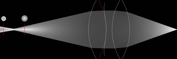
Consider a simple lens and film-plane set-up as in the figure below. Each lens1 has a certain focal length, which describes where all rays that are parallel to the z-axis will bundle. If the film-plane is placed at the focal-length we have effectively focused at objects that are infinitely far away. However if we move the film-plane closer to the lens instead of bundling rays that are infinitely far away we are know bundling rays from a finite distance away. This distance is described by the plane of focus. Any point on that plane will be projected onto exactly a single point on the film-plane.

This dependency between the film-distance and the plane of focus is described by the gaussian lens equation:
$$ \frac{1}{filmdistance} - \frac{1}{objectdistance} = \frac{1}{focallength} $$
Note that if the object distance is set to $ - \infty $ the focal distance is equal to the focal length. As the incoming rays are parallel to the z-axis und thus bundle in the focal point which as we defined earlier sets the focal length.
However if the object in the scene is not on the plane of focus different points on the lens may intersect with different parts of the object or even other objects. Or if we reverse the logic a single point in the scene now contributes to a whole area on the film-plane instead of a single pixel.
As each sample only considers a single position on the lens we need large number of samples per pixel in order to accurately consider all positions on the lens and thus possible different objects that may contribute to this single pixel.

Now we know that a point that does not lie on the plane of focus is imaged to a area on the film plane. In the case of the thin-lens model it would be imaged to a disk. Next we need to consider how large this disk appears on the film plane. This depends on both the distance of the object as well as the size of the lens which is commonly revered to as aperture. If the lens was infinitely small all rays would pass thorough it’s center and will not change their direction. As all rays from a single point hit the same point in the scene all objects appear to be in focus. In practice we refer to a object as in focus if each point on the object is projected onto a single pixel on the film-plane rather than a single point. This means that rather than considering the plane of focus as an actual plane in most circumstances we can associate a region around this plane to be in focus. As the aperture width of the field that is in focus most real lenses allow the user to reduce the lens radius by covering larger parts of the lens. The relation between the objects distance, lens aperture and the resulting radius of the disk of confusion is described by:
$$ \frac{lensdiameter}{filmdistance} = \frac{bokehdiameter}{| ; focallength - filmdistance :| } $$
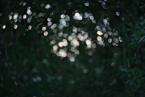
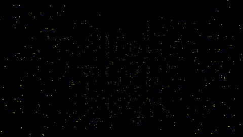
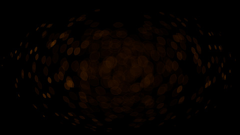
While the circle of confusion results in a blurry image in most scenes, as each pixel is getting information from many different parts of the scene . However if the image is mostly dark and there are some bright points these bright points are being projected onto the film-plane without overlapping other information. As a result the disk that this bright point is being projected to is clearly visible. It is this effect that is commonly known as bokeh.

Notice that in the lower part of the image there is generally very little light. Thus the “disk” each light-point is projected to is clearly visible as no other information overlaps with it. However in the sky there are no single bright points so the projection-disks of the different points in the sky overlap creating a blurry image.
Types of real bokeh
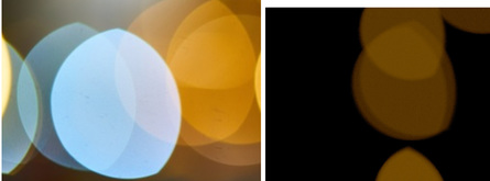
Here is a small gallery of real photos with bokeh.


From observing these and other images we notice the following properties:
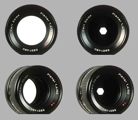
If the lens aperture is reduced by blades the bokeh can take on the form of the blades that were used. For example the first image was clearly taken with a camera lens with 6 slightly rounded blades.
When the lens is wide open the shape of the bokeh is not only depending on the aperture of the lens but also the lens housing. This effect can more easily understood when considering the image on the right. Further we can see that we can prevent optical vignetting by using the aperture blades to reduce the aperture to a point where it is independent of the lens housing. In the center of the image the rays can go into the scene without being obstructed by the lens housing resulting in a perfect sphere. The closer we get to the edge of the image the more of the circle of confusion is obstructed. This effect is further considered below.
- Manufacturing aspheric lenses often leads to a onion like carving pattern which can be seen in the bokeh.
Since pbrt does not model lens housing and uniformly samples the lens non of these effects can be achieved with the default implementation. In this implementation i have addressed the first 3 issues and i will give an approach for the 5th issue.
Starting point
PBRT uses samplers to generate well distributed sample points in the unit-square which can then be used to generate a uniform samples on the lens. Thus if we once again reverse the mental image, each point that is out of focus contributes to all points on the lens and thus creates a disk on the film plane as the rays are focused in front or behind the film-plane. To map uniformly distributed sample points in $[0-1]^2$ to a disk that is also uniformly distributed the book suggests the following approach:
Point2f ConcentricSampleDisk(const Point2f &u) {
// Map uniform random numbers to $[-1,1]^2$
Point2f uOffset = 2.f * u - Vector2f(1, 1);
// Handle degeneracy at the origin
if (uOffset.x == 0 && uOffset.y == 0) return Point2f(0, 0);
// Apply concentric mapping to point
Float theta, r;
if (std::abs(uOffset.x) > std::abs(uOffset.y)) {
r = uOffset.x;
theta = PiOver4 * (uOffset.y / uOffset.x);
} else {
r = uOffset.y;
theta = PiOver2 - PiOver4 * (uOffset.x / uOffset.y);
}
return r * Point2f(std::cos(theta), std::sin(theta));
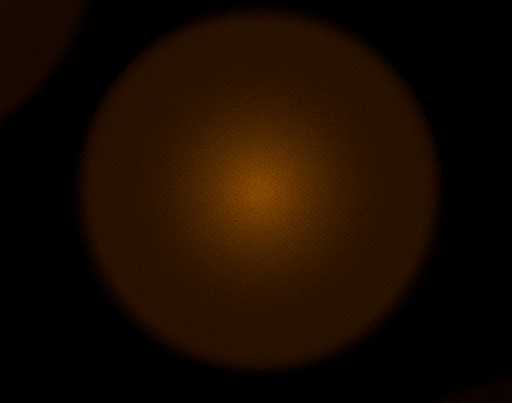
}As expected this results in uniform disk shaped bokeh:
However if we were to let’s say half the radius, r*=0.5, we effectively reduce the aperture as
a the iris would in a real lens. Analog to real photography this will reduce the depth of field as well
as the size of the circle of confusion as the “lens diameter” in the above formula get’s reduced.


Creating arbitrary blade configuration
Instead of just reducing the aperture and maintain a perfect circle we can also alter the shape as a nth-bladed iris would. Notice that such a iris will always produce a regular polygon. As each n-regular polygon can be created by using n triangles we only need to find a method to uniformly sampling a triangle in order to uniformly sample any regular polygon.
As described by Graphic Gems (p. 24) provides us with the following algorithm:
Point2f A,B,C; // points of the triangle
float s1,s2; // sample point x,y  [0-1]
return (1 - sqrt(s1)) * A + (sqrt(s1) * (1 - s2)) * B
                + (sqrt(s1) * s2) * C;
Depending on the number of blades we need to create n-triangles and figure out the vertices of each triangle. As the vertices stay the same throughout the whole rendering process we can compute them once at start up. The process is straight forward we choose a starting point that is on the unit-circle and simply rotate that point until we have n-vertices.
void initBokehVerts(Bokeh &bokehOptions) {
    int nVert = bokehOptions.blades;
    if (nVert < 3) // we need at least a triangle
        return;
    bokehOptions.step = 2 * Pi / nVert;
    bokehOptions.corners = std::unique_ptr<Point2f[]>(new Point2f[nVert]);
    float cur = Pi / 2.0f; // start at (0,1) with all polygons

    for (int i = 0; i < nVert; i++) {
        bokehOptions.corners[i] = Point2f(std::cos(cur), std::sin(cur));
        cur += bokehOptions.step;
    }
}
In our mapping code we can use those corners to generate uniform distribution within each triangle of the polygon. First we need to figure out which triangle of the polygon we are about to sample. We are simply using the first value of our lens-sample-value. Further we must clamp the value for the rare case that the sample value is exactly 1.0, which may or may not actually be generated depending on the sampler-implementation.
int index = static_cast<int>(pLens.x*bokehOptions.blades);
index= std::min(index,bokehOptions.blades -1);
However in order to maintain uniform distribution within the chosen triangle and prevent any correlation we then need to normalize the sample.
float r1 = (pLens.x-(index* (1.0f/bokehOptions.blades)))
            *bokehOptions.blades;
int previous = index + 1 == bokehOptions.blades ? 0 : index + 1;
Point2f A = Point2f(0, 0);
Point2f B = bokehOptions.corners[index];
Point2f C = bokehOptions.corners[previous];

Float r2 = pLens.y;
ret = (1 - sqrt(r1)) * A + (sqrt(r1) * (1 - r2)) * B + (sqrt(r1) * r2) * C;
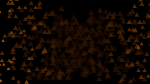
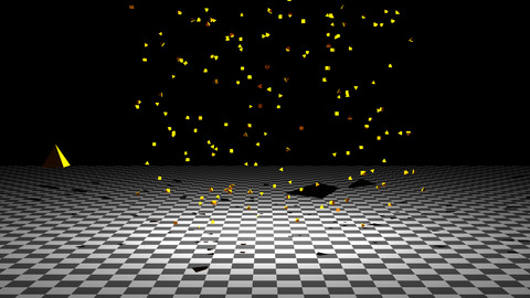
The following images show the results of this operation. How to generate the pronounced edges visible in every second image will be discussed later.


Optical vignetting
Suppose we could put a tiny camera on the film-plane of our bigger camera, this would allow us to see exactly what each pixel on the film-plane of the bigger camera would “see”. In the first scenario below our tiny camera looks through a lens where the inner radius (in red below) of the lens housing and the outer radius of the house lensing are equal in diameter. When i talk about the radius inner and outer housing what i really mean is radius of the two annulus that block the view into the scene of our tiny camera. In a wide open camera this may actually be the lens housing, in other scenarios either the inner or outer housing may be represented by iris-blades of the aperture.
The tiny camera starts at the center of both the film-plane and the lens. Both housings are projected onto the same area disk like area onto the film-plane as evident by the white circle at the start of the video below. However if we move our tiny camera to the left of the film-plane of our bigger camera we notice that the projection of housing is being shifted unequally as such the intersection of both projections forms the view into the scene from that pixel.
In the next scenario we only changed the diameter of the inner lens housing (red). Right when we start at the center of the film-plane we already notice a difference to the previous scenario. Unlike before the shape of the projection now only depends on the outer diameter. Only when we get to the very outer edge of the image the inner lens housing obstructs part of the outer radius.
In the last scenario we decreased the diameter of inner housing. Once again we the shape of the projection is depending on the inner housing for most of the pixels on the film plane. Only the outer pixels are effected by the outer lens housing.


Notice that in each scenario we can model the lens housing by using the intersection of two circles. Further we can reason that if we move the outer lens housing further back it would still project to a disk though a smaller one. Thus we can represent the projection area of any lens by the intersection of two circles of different sizes3 . If the ratio between the circle is around 1.0, both inner and outer lens housing have the same diameter, we can recreate the first scenario. If we change this ratio we can recreate the other two scenarios. So all we need to know to model the bokeh is the ratio between the projection of the inner housing onto the film plane and the projection of the outer lens housing. To recreate this effect simply move the inner circle depending on the film-plane position. We can further model the size of the film plane by reducing the amount that we move the inner circle. This is equivalent to limiting the movement of our tiny camera to a smaller region. First we map the samples to the unit-sphere as this represents the largest opening of our camera. We then proceed to cut away some of it’s light due to optical vignetting. While it is physically plausible that the outer regions of the image receive less light (rays) it may be cause performance problems especially on gpus.
float rateOfChange,radius; // user controlled parameters
Point2f s = ConcentricSampleDisk(sample.pLens);
// fixed circle
float c1 = s.x * s.x + s.y * s.y;
// convert film samples to [0-1]
Point2f ndc = sample.pFilm;
ndc.x /= film->fullResolution.x;
ndc.y /= film->fullResolution.y;
ndc.y = 1.0f - ndc.y;
// convert to [-1,1]
ndc = 2.f * (ndc) - Vector2f(1, 1);
s.x += rateOfChange * ndc.x;
s.y += rateOfChange * ndc.y;
float c2 = s.x * s.x + s.y * s.y;
c2 *= radius; // controls the shape
// reject samples that are not in the overlapping area
if (c1 >1 || c2 > 1)
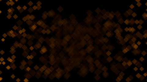
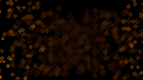
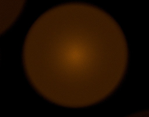
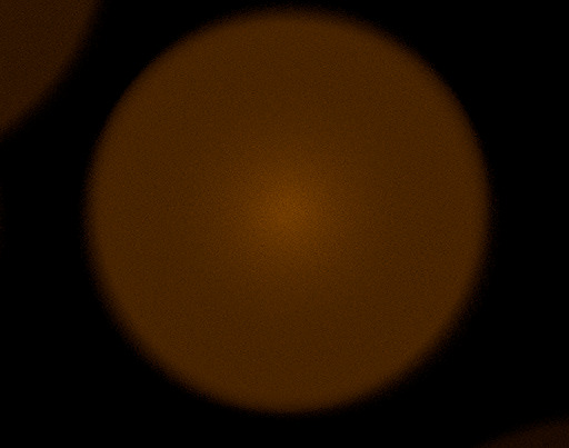
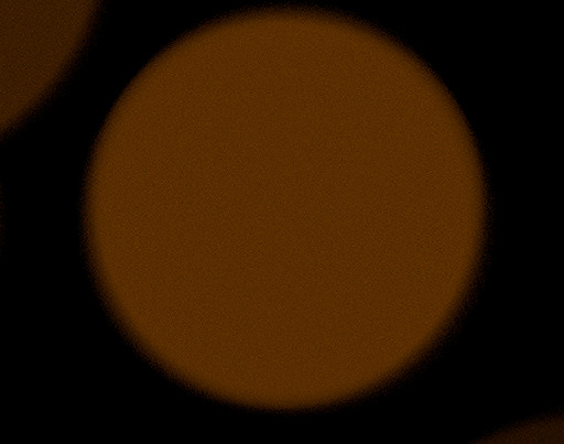
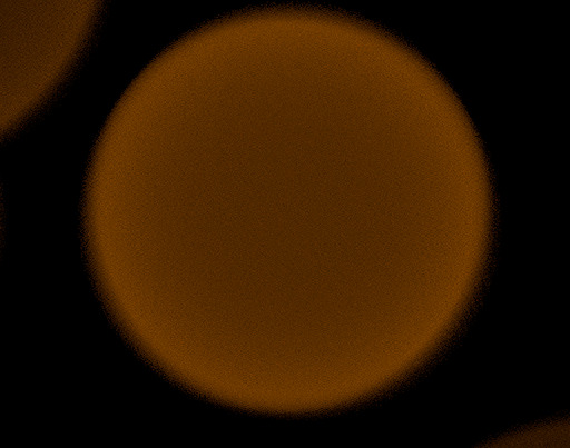
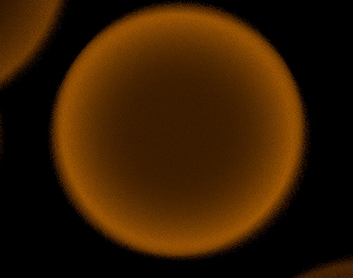
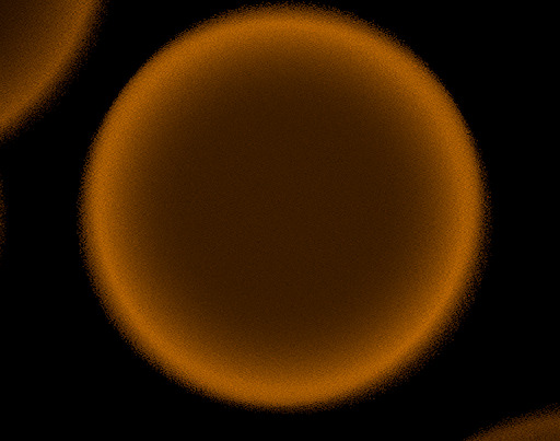
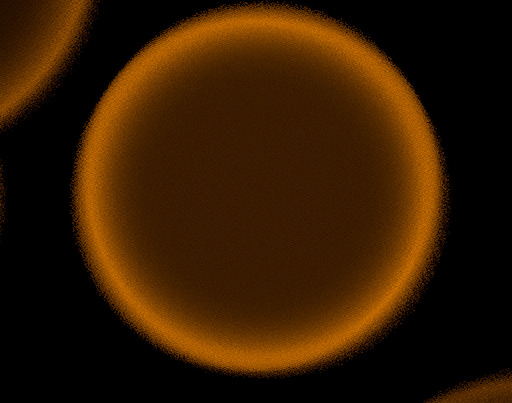
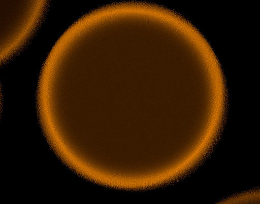
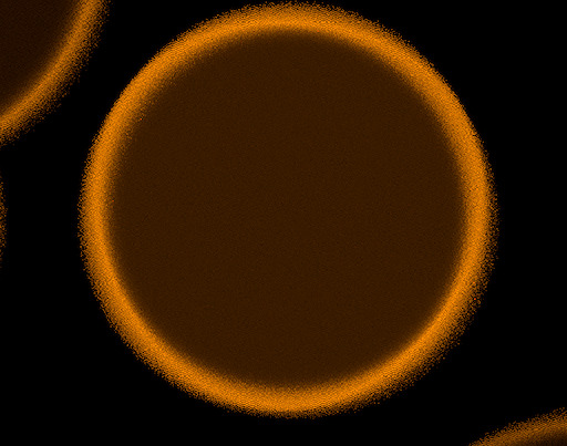
weight = 0.0f;We can see the resulting shape in the following images. Varies from 0.2 in the first image to 2 in the last two images. The last image demonstrate that the distortion has no effect when the image is rendered with a lens radius of 0.


Creating a pronounced edge for the bokeh
Properties 3 to 5 can all be realised by altering the weight of each sample depending on their position. From these the pronunciation of edges was chosen to be implemented.
So we need a way to check if the sample is on the edge of the bokeh shape. For the default implementation which always creates a perfect disk this is easy. We can use the distance to the center to determine if the sample is on the edge of that disk. What is and what is not edge is defined by the input-file. A value of 0 would be mean the whole circle is the edge, thus no weights are altered. A value of 1 would reduce the values of all samples. For most purposes a value between 0.8 and 0.95 works well. The edgeStrength determines how pronounced the edge will be, or in other words how much the value that do not count as edge are reduced by.

// << ADD TO DISK CODE >>
edge = std::abs(r);
// << ADD TO POLYGON CODE >>
edge = r1;
// << ADD TO OPTICAL VIGNETTING CODE >>
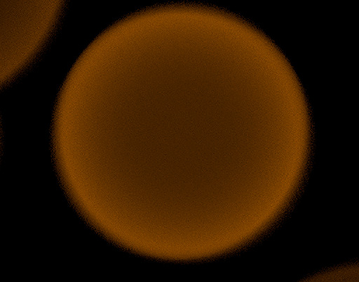
edge = std::max(c1, c2);After we have calculated the “radius”-value for each shape we can apply a weighing function to create the desired distribution. For this i use the function below with parameters for distribution (d) and the strength (p). I added a balance term $ - \frac{p}{d+1} $ to ensure the total amount of light going through the bokeh shape will not be altered.
I choose to display the range from -1 to 1 be displayed as it is easier to imagine the bokeh distribution
that will be generated from the distribution that way. However as seen before we are actually using a unsigned
distance for x which means $ x \in [0,1] $ which further allows us to use a continuous scale for $d$ instead of
stepsize of 2 as in the diagram above. If the user supplies a negative value for d the bokeh shape is inverted
by x = 1-x;. Some values are precomputed at start up otherwise it is a direct implementation of the above function
and thus not included here. Further the value of p will be scaled with d+1 which makes for a more intuitive strength
control between [0,1]. The user can set other values but will get a warning that values above one will result in
light-loss.
For the first 5 image we fix the distribution at -4 and alter the strength from 0.8 to 0. The next 5 image fix the distribution at 4 and alter the strength as before. The last 5 fix the strength at 0.6 and alter the distribution to $5.5,8.7,12.7,20.7,50.7$ .

Manufacturing and imperfections
As discussed before the manufacturing process can leave a carving pattern on the lens. This could be easily be implemented by using a additional user-specified weight map which captures those carving patterns as well as any other imperfections on the lens.
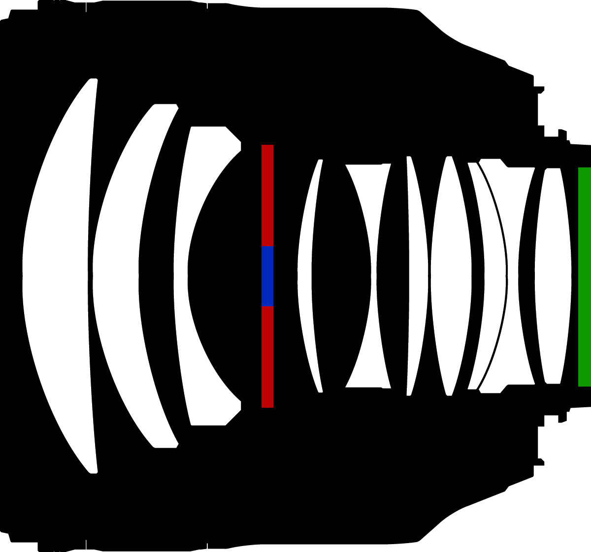
Alternatives
PBRT it self offers a alternative to create the correct bokeh form with the realistic-camera implementation. The realistic camera takes a lens description which includes the curvature radius, thickness, index of refraction and aperture diameter of each lens element. This produces a more realistic bokeh form for a specific this lens input file. However many lenses are made up of 8 or more lens-elements as such to create a specific bokeh form the values for each element need to be set accordingly which in turn effect focal length of the lens. In other words it is fairly difficult to alter the shape of the bokeh. In comparision my approach offers four control slide to effect both shape and light distribution making it easier to interact with the model.
File format integration
The changes have been integrated with with the file format and can be used in conjunction with the perspective and realistic camera. Other camera types are unaffected by these parameters and work as if they had not been specified.
| Type | Name | DefaultValue | Description |
|---|---|---|---|
| int | lenselements | 0 | How many blades are used in the lens aperture. 0 indicating a perfectly round iris. |
| float | lensRatio | 1.0 | Relative radius of the inner obstructing sphere |
| float | rateOfChange | 0.0 | Controls how much the projection differs from a perfect circle. |
| float | weightDistr | 0.0 | Controls which amount of the bokeh is not part of the edge. |
| float | weightStrength | 0.5 | Amount by which the position which are not part of the edge are reduced. |
The default values will leave old scenes unaltered as they do not change the systems behavior.
1. For now we assume a perfect thin lens-model which only a single element. ↩
2. Outer as in further away from the film-plane. Analog inner radius as in closer to the film-plane. ↩
3. We ignore the effect that the lens housing may be distorted to a ellipse as this would as this effect only occurs if the film plane is very close to the inner lens radius or the film plane is significantly larger as depicted in the figure. ↩
All used image are licenced through a CC0 licence or rendered using custom scenes with the pbrt-render system .